
Pratiman Patel, 05 August 2021
3 min read.Using MetPy as straightforward as possible to make a Skew-T LogP plot for WRF out file.
import wrf
from netCDF4 import Dataset
import matplotlib.pyplot as plt
import proplot as pplt

import metpy.calc as mpcalc
from metpy.plots import SkewT
from metpy.units import units
wrfin = Dataset(r'wrfout_d01_2017-06-08_00_00_00')
lat_lon = [48.856, 2.352]
x_y = wrf.ll_to_xy(wrfin, lat_lon[0], lat_lon[1])
p1 = wrf.getvar(wrfin,"pressure",timeidx=0)
T1 = wrf.getvar(wrfin,"tc",timeidx=0)
Td1 = wrf.getvar(wrfin,"td",timeidx=0)
u1 = wrf.getvar(wrfin,"ua",timeidx=0)
v1 = wrf.getvar(wrfin,"va",timeidx=0)
p = p1[:,x_y[0],x_y[1]] * units.hPa
T = T1[:,x_y[0],x_y[1]] * units.degC
Td = Td1[:,x_y[0],x_y[1]] * units.degC
u = u1[:,x_y[0],x_y[1]] * units('m/s')
v = v1[:,x_y[0],x_y[1]] * units('m/s')
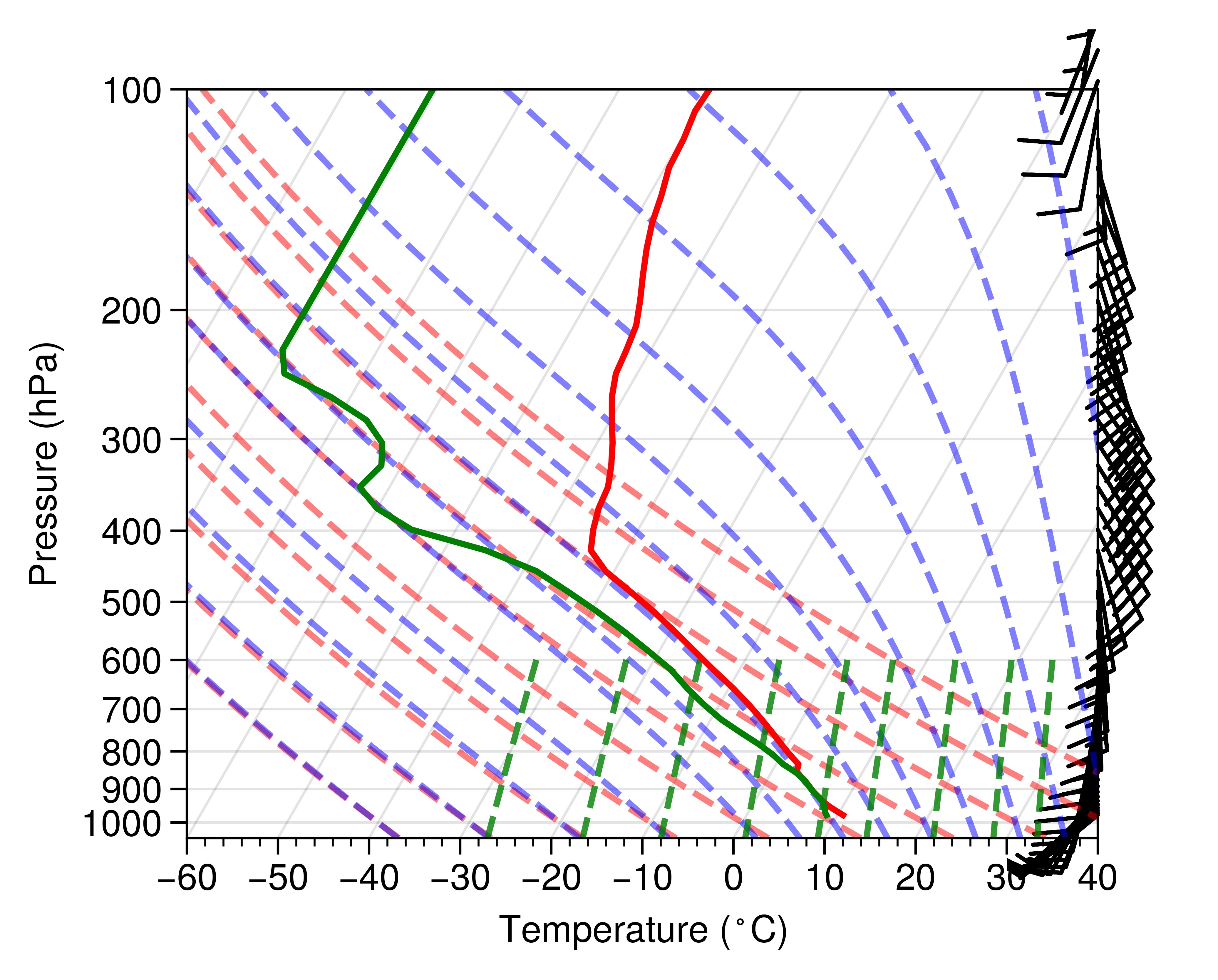
skew = SkewT()

# Plot the data using normal plotting functions, in this case using
# log scaling in Y, as dictated by the typical meteorological plot
skew.plot(p, T, 'r')
skew.plot(p, Td, 'g')
skew.plot_barbs(p, u, v)

# Add the relevant special lines
skew.plot_dry_adiabats()
skew.plot_moist_adiabats()
skew.plot_mixing_lines()
skew.ax.set_xlim(-60, 40)
skew.ax.set_xlabel('Temperature ($^\circ$C)')
skew.ax.set_ylabel('Pressure (hPa)')

plt.savefig('SkewT_Simple.png', bbox_inches='tight')
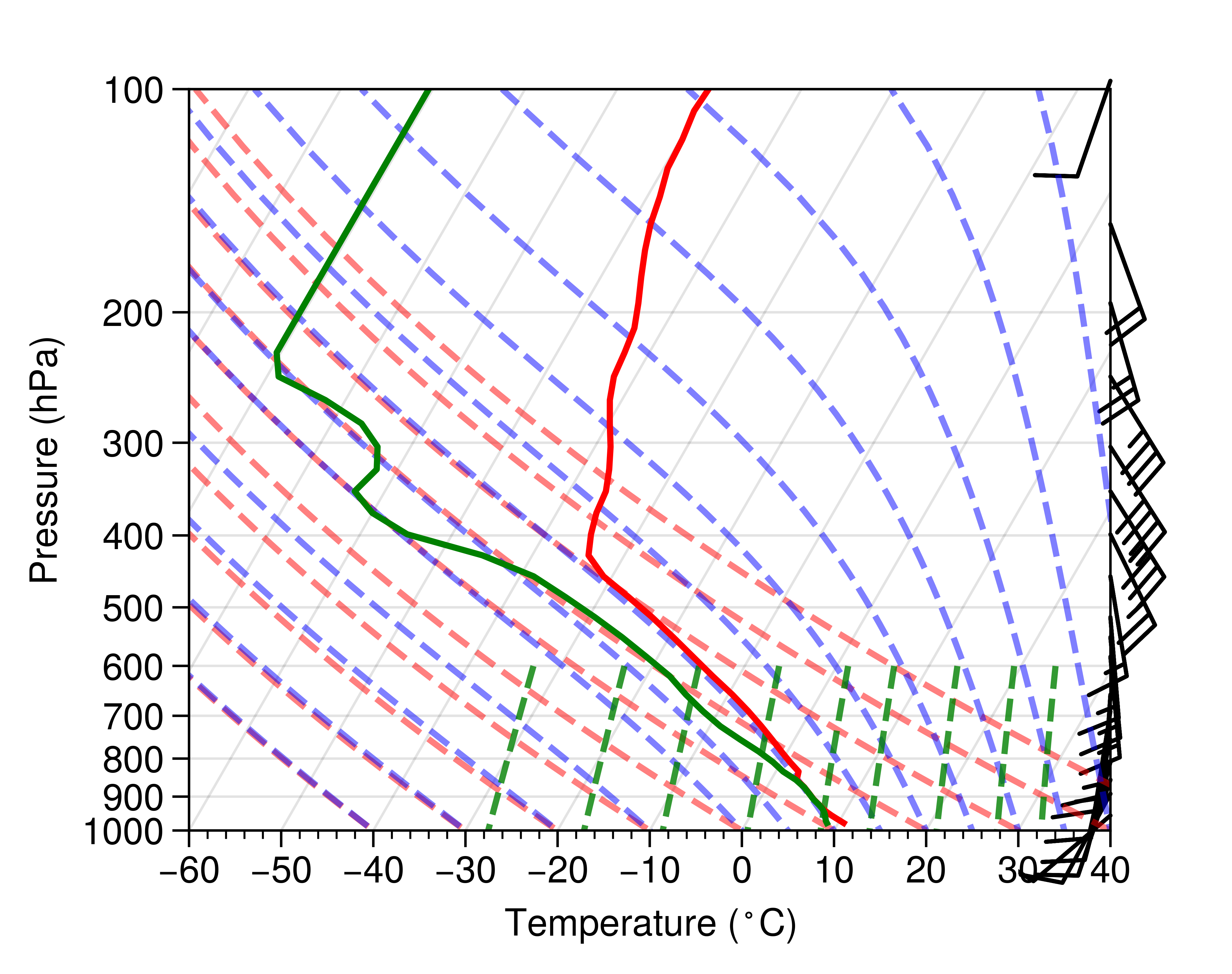
# Example of defining your own vertical barb spacing
skew = SkewT()

# Plot the data using normal plotting functions, in this case using
# log scaling in Y, as dictated by the typical meteorological plot
skew.plot(p, T, 'r')
skew.plot(p, Td, 'g')

# Set spacing interval--Every 50 mb from 1000 to 100 mb
my_interval = np.arange(100, 1000, 50) * units('mbar')

# Get indexes of values closest to defined interval
ix = mpcalc.resample_nn_1d(p, my_interval)

# Plot only values nearest to defined interval values
skew.plot_barbs(p[ix], u[ix], v[ix])

# Add the relevant special lines
skew.plot_dry_adiabats()
skew.plot_moist_adiabats()
skew.plot_mixing_lines()
skew.ax.set_ylim(1000, 100)
skew.ax.set_xlim(-60, 40)
skew.ax.set_xlabel('Temperature ($^\circ$C)')
skew.ax.set_ylabel('Pressure (hPa)')

plt.savefig('SkewT_Advanced.png', bbox_inches='tight')
import wrf
from netCDF4 import Dataset
import matplotlib.pyplot as plt
import proplot as pplt

import metpy.calc as mpcalc
from metpy.plots import SkewT
from metpy.units import units

wrfin = Dataset(r'wrfout_d01_2017-06-08_00_00_00')
lat_lon = [48.856, 2.352]
x_y = wrf.ll_to_xy(wrfin, lat_lon[0], lat_lon[1])

p1 = wrf.getvar(wrfin,"pressure",timeidx=0)
T1 = wrf.getvar(wrfin,"tc",timeidx=0)
Td1 = wrf.getvar(wrfin,"td",timeidx=0)
u1 = wrf.getvar(wrfin,"ua",timeidx=0)
v1 = wrf.getvar(wrfin,"va",timeidx=0)

p = p1[:,x_y[0],x_y[1]] * units.hPa
T = T1[:,x_y[0],x_y[1]] * units.degC
Td = Td1[:,x_y[0],x_y[1]] * units.degC
u = v1[:,x_y[0],x_y[1]] * units('m/s')
v = u1[:,x_y[0],x_y[1]] * units('m/s')

# Example of defining your own vertical barb spacing
skew = SkewT()

# Plot the data using normal plotting functions, in this case using
# log scaling in Y, as dictated by the typical meteorological plot
skew.plot(p, T, 'r')
skew.plot(p, Td, 'g')

# Set spacing interval--Every 50 mb from 1000 to 100 mb
my_interval = np.arange(100, 1000, 50) * units('mbar')

# Get indexes of values closest to defined interval
ix = mpcalc.resample_nn_1d(p, my_interval)

# Plot only values nearest to defined interval values
skew.plot_barbs(p[ix], u[ix], v[ix])

# Add the relevant special lines
skew.plot_dry_adiabats()
skew.plot_moist_adiabats()
skew.plot_mixing_lines()
skew.ax.set_ylim(1000, 100)
skew.ax.set_xlim(-60, 40)
skew.ax.set_xlabel('Temperature ($^\circ$C)')
skew.ax.set_ylabel('Pressure (hPa)')

plt.savefig('SkewT_Advanced.png', bbox_inches='tight')