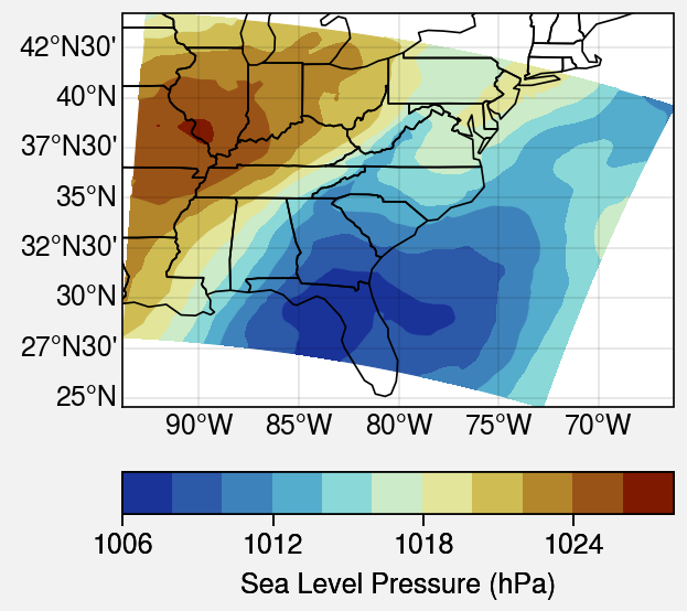
Here is an example of generating a surface plot from WRF output file. I find this method to be more elegent.

Python Script

import wrf
from netCDF4 import Dataset
import proplot as plot
import cartopy.crs as crs

# Download the dataset from https://www.unidata.ucar.edu/software/netcdf/examples/wrfout_v2_Lambert.nc
# Load the dataset
ncfile = Dataset('wrfout_v2_Lambert.nc')

# Get the variable
slp = wrf.getvar(ncfile, "slp")

# Get the latitude and longitude points
lats, lons = wrf.latlon_coords(slp)

# Get the cartopy mapping object
cart_proj = wrf.get_cartopy(slp)

#Plotting
fig, axs = plot.subplots(proj=cart_proj)

# Define extents
lat = [lats.min(), lats.max()]
lon = [lons.min(), lons.max()]

#format the plot
axs.format(
    lonlim=lon, latlim=lat,
    labels=True, innerborders=True
)

#Plot using contourf
m = axs.contourf(wrf.to_np(lons), wrf.to_np(lats), wrf.to_np(slp), 
                      transform=crs.PlateCarree(), cmap='roma_r')

#Adding colorbar with label
cbar = fig.colorbar(m, loc='b', label='Sea Level Pressure (hPa)') 

#Saving the figure
fig.savefig('slp.png')

Output

Explanation

1. Basic import stuff for Python

   import wrf
   from netCDF4 import Dataset
   import proplot as plot
   import cartopy.crs as crs
   

2. Loading the dataset

   ncfile = Dataset('wrfout_v2_Lambert.nc')
   

3. Extracting the varibale of your choice. Here it is sea level pressure (SLP).

   slp = wrf.getvar(ncfile, "slp")
   

4. Get the lat/lon and projection of the WRF file. Here the projection is LCC.

   lats, lons = wrf.latlon_coords(slp)
   cart_proj = wrf.get_cartopy(slp)
   

5. Create the plot and define projection using proj.

fig, axs = plot.subplots(proj=cart_proj)

1. Setting up the extent of the plot by getting the maximum and minimum lat and long.

   lat = [lats.min(), lats.max()]
   lon = [lons.min(), lons.max()]
   

2. Format the plot aesthetics.

   axs.format(
    lonlim=lon, latlim=lat,
    labels=True, innerborders=True
   )
   

3. Plot the filled contour of the variable.

   m = axs.contourf(wrf.to_np(lons), wrf.to_np(lats), wrf.to_np(slp), 
                      transform=crs.PlateCarree(), cmap='roma_r')
   

4. Adding the colorbar at the bottom of the plot.

   cbar = fig.colorbar(m, loc='b', label='Sea Level Pressure (hPa)') 
   

5. Finally, saving the figure.

   fig.savefig('slp.png')
   

Additional Information

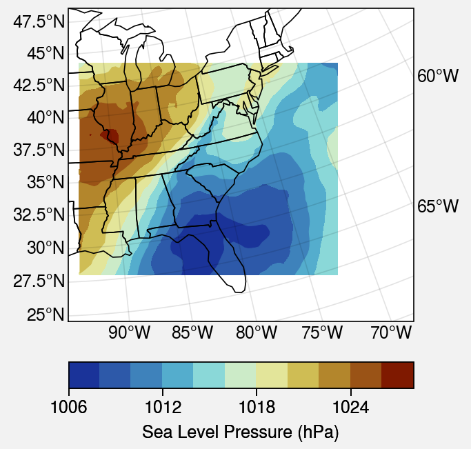
If you do not like the LCC projection then you can change the following line:

fig, axs = plot.subplots(proj='cyl')

Output